


The statistical significance of Fundamental Factors
How to understand overfitting in the context of fundamental factor models - and in particular why most modellers use t-value cut-offs

In this post we’re going to take another look at the daily regressions performed in fundamental factor models. By deriving the distribution of estimated returns for each day, we will look at the distribution of t-stats through time, showing why modellers analyse the distribution of daily factor t-stats to assess whether to include regression factors in their models. We show that factors which have high t-stats, even for a relatively low portion of days, are unlikely to be false positives when testing reasonable numbers of factors.
As with last week, this post is probably somewhat more technical than the average post will be. Normal service will be resumed shortly!
In the previous post, we discussed why higher R-squared is considered valuable in fundamental factor models. One caveat mentioned at the time was the risk of overfitting -as adding more factors to the model will automatically increase R-squared, even if the factor added doesn’t correspond to any real market factor.
This is a significant risk with all models, particularly statistical models: random matrix theory tells us that any estimated covariance matrix will show certain sets of variables as appearing correlated, even if all the variables are actually independent. Risk modellers often apply shrinkage to estimated covariance matrices to deal with this problem, reducing the risk of the largest concentrations of risk and increasing risk in the broad matrix.
As discussed in the last post, fundamental factor models are essentially already operating an unusually-structured shrinkage methodology - first a modeller decides that all cross-security factors must be related to observable security characteristics, then they take the set of all observable characteristics and selecting a subset of those factors to use for risk estimation. Once done, they then assume no cross-security correlation outside of this.
However, this begs the question: of all the many hundreds of potential observable factors, how should a modeller select a good set of factors from our forest of potential factors? It’s clear that just adding a new factor increases explanatory power - but what tests can be used to determine when to add or discard a particular factor? This is a particularly tricky question when analyses are generally all done in-sample, using all the available data.
Daily Factor Return Regressions: More Than You Wanted To Know
To have faith that they have chosen a true factor, the analyst has to have faith that the where a factor’s returns persistently show statistical significance, it is statistically likely that this is because of a true underlying relationship.
To understand this, let’s take a deep dive into the regressions that determine the daily returns of each individual factor. Without (much) loss of generality, let’s assume that we’re operating with a market which is characterised as follows1:
We can write this in matrix notation as follows2:
Each daily returns regression gives us an estimate for this factor return vector. To understand significance of each factor, we want to understand both the expected factor returns and their distribution3:
So far, we’ve not made any assumptions about the distributions of the various factor exposures that we’re inputting. To make this easier to think about, we’re going to assume that each of our input exposure vectors are independent factors4 with zero mean exposure5. In this case:
Those who have spent time with regressions will recognise that this is a rederivation of the standard error.
What Does This Have To Do With The Regression T-Stat?
To understand the t-stat, firstly we want to look at the distribution of the fitted factor returns we will expect to see. Our fitted returns will have an ex-ante distribution with an expectation equal to the true mean returns, but with higher variance due to the estimation error.
In the case where our true factors are normally distributed6, this looks as follows7:
Since the standard error is essentially a scalar, using the sample standard error, we can approximate the distribution of the t-stats as8:
What Does This Mean For Testing For Overfitting?
The above distribution of the fitted t-stats should immediately show why modellers look at the estimated t-stat.
Spurious factors by definition have a true mean return of zero, as well as zero true variance; for these factors the ex-ante distribution of the fitted t-stat collapses to a normally distributed variable with mean zero and sigma 1.
By contrast, true factors will have t-stats should either have non-zero true mean or higher-than-unit true standard deviation. The higher the absolute return to the factor or the higher its true factor risk relative to the market’s general level of idiosyncratic risk, the higher the absolute mean and standard deviation of the daily t-stats will be.
Factor modellers tend to only choose factors with at least a certain proportion P of t-stats higher than some cut-off C. These cut-offs can be calibrated to give a desired proportion of type-one versus type-two errors.
In practice, factor modelling companies tend to use a cut-off of 2 for a relatively small proportion of days. For a randomly chosen vector of exposures with no true factor correlation, assuming normality, the chance of a single day’s absolute t-stat being greater than 2 is 4.55%. We can use the binomial distribution to estimate the probability that a particular factor will generate a false positive on a given number of days, and with that calculate the probability that multiple tests will generate at least one false positive.9
As such, for a model calibrated over 500 datapoints10, we get the following probability of a type II error at different thresholds when testing for multiple factors:
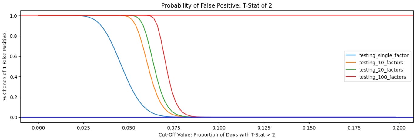
Even for a very large number of simultaneous tests, the odds of having t-stats persistently higher than the threshold is low. Setting a cut-off at 20% of days or even 10% of days allows modellers to exclude most totally spurious factors, and setting a relatively low threshold allows true factors with episodic or time-varying volatility or mean.
Avoiding overfitting in factor selection while ensuring that real factors are not excluded is an exercise in balancing type one errors - incorrectly accepting false factors - and type two errors, where you incorrectly reject true factors. The chart above only shows that our t-stat cut-off has a high probability of avoiding type one errors by rejecting false factors. A full analysis would also show the probability of falsely rejecting a true factor is also low. However, this probability is highly dependent on the level of factor volatility relative to idiosyncratic volatility and the distribution of the underlying factor, and doesn’t have a neat closed-form description. We’ll consider this analysis in a follow-up piece.
An Alternative Vector Space Explanation
An alternative way of thinking about the question of correct factor selection is in vector space. Of all the true and spurious factors with statistical significance in the market, what is the probability a given technique has accepted one of the true factors versus one of the spurious factors? Again, while analysing the chance of a type two error is highly dependent on the structure of true factors, we can consider the chance of a type one error much more easily.
The returns distribution of a market of n securities can be thought of as an n-dimensional covariance space. Because they are defined by baskets of securities, each candidate fundamental factor reflects a vector within the space. Every time we trial a new factor within the space, we increase the dimension of the subspace which is covered by the model.
Once we have captured all of the true security-level covariance with our existing f factors in the space, we assume that the true variance along any of the other n-f dimensions in the space is the same - there’s no vector which has higher true variance than any other.
We know from random matrix theory that empirically, it will appear that some vectors will have more variance in them than others. we could identify these by - for example - principal components analysis, which will simultaneously look at all the remaining n-f dimensions and identify the highest-empirical-variance vectors. If we use this vector in a fundamental factor model, we will likely have found a vector which looks significant!
Is this a problem for a fundamental factor modeller? Yes - but it is much less of a problem for that modeller than it would be for someone using a statistical model. The statistical modeller has a probability of 1 of finding the highest variance vector, because they are testing every single vector and selecting the largest; by contrast, a fundamental factor modeller testing g new factors only has g/(n-f) chance of finding the highest variance factor. As long as they are disciplined about the number of factors they test, they limit their chance of finding spurious factors.
For each date and security, the return is equal to the sum of the market factor return (signified by beta_jt), multiplied by each security’s exposure to that factor at time t (x_ijt), plus a stock-specific idiosyncratic return (epsilon_it). The specific assumption of homoskedasticity - identical variance of the error terms - is unnecessary but convenient; where any heteroskedasticity is known, this can be adjusted for by using a weighted regression approach
This is a near-identical formulation to the previous one - we’ve switched from describing returns at the individual security level to the level of the market, and been more precise about the distribution of the idiosyncratic return of the individual securities, which will form the regression error term
This is a standard estimate from an OLS regression, showing the expected regression betas and their variance
As far as the assumption of independence is concerned, in practice analysis is conducted on highly-correlated factors individually. Often such factor exposures are aggregated together, particularly where there is a fundamental reason to assume they are related. For example, most models’ value factors will be an average of price to book, price to earnings and potentially other similar factors. This can be considered an extremely primitive form of regularisation.
This is usually the case for style factors by construction, as modellers usually use z-scores; it is usually not true for industry dummy factors, where the average exposure is usually equal the proportion of securities in the universe which have a loading.
The assumption that input factor returns are normally distributed is unnecessary but helpful. The standard error of the estimate is normally distributed even if idiosyncratic and factor returns aren’t normally distributed, as long as sufficient datapoints are available that the Central Limit Theorem is applicable, and exposures are distributed in a certain ways which are generally true about the exposure vectors used in fundamental factor models. However, assuming the true factor returns are normally distributed makes the distribution of fitted returns convenient to specify.
Looking at this equation shows that the risk of the estimated factor return series should be slightly higher than the true risk of the factor - usually this is handled by a small adjustment to factor returns to remove the contribution from this estimation error
A proper adjustment for standard error would slightly change this equation, increasing both variance
Properly adjusting for reducing degrees of freedom in the regression slightly complicates this, meaning the true probability of getting a false positives for multiple tests is slightly higher than an assumption of independence would indicate, but in larger markets this effect should not be encountered by the following simulation
This can be considered as 2 years of daily data, 10 years of weekly data, or around 20 years of rolling monthly data - all very possible with modern market data